Project Laminar
Beating Schwab Intelligent Portfolios with ease.
Normalizing flows for generative modeling of tabular datasets.
This library provides tools for generative modeling of tabular datasets using normalizing flows. Some of its core features include:
To get started with EchoFlow, check out our documentation!
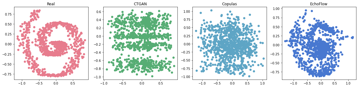
Let us start by considering a simple tabular dataset containing two columns which, when plotted, forms a spiral. Our goal will be to train a generative model on this dataset and then sample from it to create a "synthetic" copy of the dataset. Some of the tools for accomplishing this include:
We applied each of these methods to our spiral dataset, generated 1000 samples, and visualized the results below.
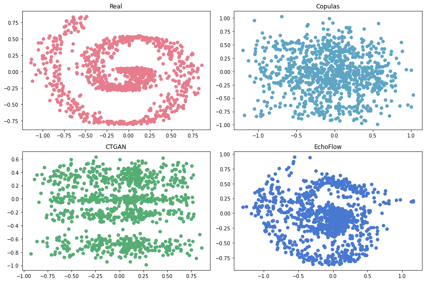
As shown in the above figure, EchoFlow produces significantly higher quality samples than either Copulas or CTGAN. In the following sections, we will (1) introduce some of the key concepts and math behind normalizing flows and (2) demonstrate some of the core functionality provided by the EchoFlow library.
At a high level, normalizing flows work by transforming random variables with invertible neural networks by applying the change of variables in the probability density functions.
The most important property of a normalizing flow is that it must be invertible. In practice, this means that each layer of the neural network must be invertible so that the whole neural network can be inverted.
This property is critical because the direct pass - \(f(x)\) - is used to map the input distribution to the prior distribution and the inverse pass - \(f^{-1}(z)\) - is used to map the prior distribution back to the target distribution.
For example, given a trained network, the direct pass could be used to map your tabular data to a standard multivariate normal distribution to evaluate the log-likelihood. Using the same network, the inverse pass could be used to map random noise sampled from the multivariate normal distribution into samples that resemble the original tabular data.
For those of you who are familiar with variational auto-encoders (VAE), these ideas may sound familiar - the direct pass is essentially the encoder in a VAE while the inverse pass is essentially the decoder. However, with normalizing flows, these two networks are combined into one invertible neural network.
Suppose you have a random variable \(x\) which has distribution \(p_x(x)\). If you apply a function \(z = f(x)\), then the random variable \(z\) has the following distribution:
\[ p_z(z) = p_x(x) \bigg| det \frac{\partial f}{\partial x} \bigg|^{-1} \]
Normalizing flows use a neural network as the function \(f\) and apply this change of variable formula repeatedly to get from the input distribution to the prior distribution. Then, the loss function is simply the negative log-likelihood of the data. Therefore, in addition to being invertible, our neural network needs to be designed in such a way that the determinant of the Jacobian is easy to compute.
The general strategy used to achieve this is to use neural networks that have triangular Jacobian matrices. This corresponds to a model where, assuming the network has N inputs/outputs, the \(i\)th output only depends on the preceding \(i-1\) inputs. By using this type of autoregressive structure in each layer of the network, the determinants of the Jacobians can be multiplied together to compute the likelihood.
One way to get insight into how normalizing flows work is to visualize the output of each layer. The below example shows the output of each layer in a normalizing flow network which is being trained on the spiral dataset with a Gaussian prior.
The input is a standard multivariate normal. Each layer transforms the distribution until it approaches the target distribution which resembles a spiral.
The EchoFlow library implements normalizing flows using PyTorch but also provides additional functionality to make it easier to apply to real-world tabular datasets. To get started with EchoFlow, you can install it from pip by running:
pip install echoflow
python -c "import echoflow; print(echoflow.__version__)"
Then, you can load the spirals dataset and train an EchoFlow model as follows:
from echoflow import EchoFlow
from echoflow.demo import load_dataset

model = EchoFlow()
model.fit(load_dataset())
synthetic = model.sample(num_samples=10)
You can pass any DataFrame to the fit method; the sample method will yield a new DataFrame containing the synthetic data with the specified number of rows. For advanced usage including conditional sampling, custom transformers, and more, check out our documentation here!
EchoFlow uses the SDGym library for benchmarking. Using the default models - RNVP and MADE - we obtain better results than the CTGAN model across a variety of simulated datasets.
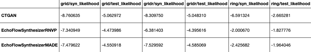
Currently, EchoFlow does not outperform the baseline on several real world datasets, largely due to sub-optimal handling of categorical values. We are looking into improving support for categorical variables through methods such as discrete normalizing flows and treating them as external conditioning variables as in CTGAN.